
Why the B-H Curve Matters More Than the Grade Datasheet
Most motor designers select a magnet grade from a datasheet, verify that Br and Hcj meet the application requirements, and stop there. This is fine for simple applications and off-the-shelf motor designs where someone else has already done the magnetic circuit analysis. It becomes a problem when the magnet geometry, air gap, or operating temperature differs from the reference design, which in custom motor development is nearly always the case.
The grade datasheet gives the magnet's intrinsic properties - what it can do in isolation. The magnetic circuit analysis tells you what it actually does in your specific design. The two numbers can be substantially different, and the gap between them determines whether your motor hits its torque target or falls short by 15% at operating temperature. This article covers the core analytical tools: the load line, the operating point, and the practical implications for design decisions.
1. The B-H Curve and What It Actually Tells You
The demagnetization curve (the second quadrant of the B-H curve) for a sintered NdFeB magnet has two key coordinates. The remanence Br is the flux density when no external field is applied (H = 0). The coercivity Hcb is the reverse field strength required to bring B to zero. Between these two points, the curve is nearly linear for modern NdFeB grades - the slope is the magnet's permeability, approximately μ₀ × μᵣ where μᵣ ≈ 1.05 for sintered NdFeB.
What the datasheet does not directly show is where the magnet will actually operate in a closed magnetic circuit. In any real application, the magnet is part of a circuit that includes the air gap, the steel components, and the geometry. The operating point - the actual (B, H) coordinate on the demagnetization curve - depends on the circuit geometry, not just on the magnet material. Two designs using the same grade in different air gap configurations will have different operating points, different flux densities in the gap, and different demagnetization safety margins.
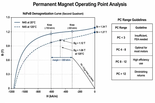
The critical boundary is the knee of the demagnetization curve. For grades without the H or SH suffix (standard NdFeB), the knee occurs at around H = −700 to −800 kA/m depending on grade and temperature. If the operating point drops below the knee - meaning the external demagnetizing field drives the magnet into this nonlinear region - the magnet partially demagnetizes irreversibly when the field is removed. For H-grade magnets, the knee is pushed to −1100 kA/m or lower, which is why they're specified for applications with significant armature reaction fields or high operating temperatures.
2. The Load Line: Connecting Magnet Properties to Circuit Geometry
The load line is the circuit's constraint on the magnet's operating point. It is a straight line drawn on the B-H plane, originating at the origin and intersecting the demagnetization curve at the actual operating point. The slope of the load line is called the permeance coefficient (PC), and it is determined entirely by geometry:
PC = (Ag × Lm) / (Am × Lg)
where Ag is the air gap cross-sectional area, Am is the magnet pole face area, Lm is the magnet length in the magnetization direction, and Lg is the air gap length. This is the simplified version assuming perfect magnetic steel (no flux leakage, no steel reluctance) - the full version adds leakage permeance terms, but this approximation is adequate for initial design decisions.
A high PC (steep load line slope) means the magnet operates closer to Br - more of the magnet's flux capacity is utilized. A low PC (shallow slope) means the magnet operates farther from Br, delivering less flux density to the gap but with more resistance to demagnetization from external fields. The typical useful range for PC in motor applications is 4–12. Below 3, you're not efficiently using the magnet. Above 15, you're using the magnet efficiently but the geometry is often impractical (very thick magnets relative to the gap).
For a radial flux motor with Lm = 5mm, Am = Ag (no fringing), and Lg = 1mm, PC = 5. If the grade is N45 with Br = 1.34 T, the operating flux density in the gap is approximately Br × PC/(PC+1) = 1.34 × 5/6 ≈ 1.12 T. This is the number that goes into the force or torque calculation, not the datasheet Br. The difference is 16% - not negligible for a close-tolerance motor design.
3. Temperature Effects on the Operating Point
Both Br and Hcj decrease with temperature. For standard N45 NdFeB, the temperature coefficients are approximately −0.11%/°C for Br and −0.55%/°C for Hcj. At a winding-adjacent magnet temperature of 120°C (50°C above room temperature reference), Br drops to 1.34 × (1 − 0.0011 × 50) = 1.27 T and Hcj drops from approximately 1150 kA/m to approximately 1150 × (1 − 0.0055 × 50) = 833 kA/m.
The operating point also shifts with temperature. Both the demagnetization curve coordinates and the load line intersect move. For most motor geometries with PC in the 4–8 range, the operating flux density drops roughly in proportion to Br - so a 5% Br drop at temperature produces approximately a 5% torque reduction. This is the standard motor thermal derating calculation.
The more dangerous effect is the shift of the knee point. At 120°C, an N45 magnet has Hcj of approximately 833 kA/m. The knee of the demagnetization curve (for the standard grade) is now at approximately H = −500 kA/m, rather than −750 kA/m at room temperature. If the motor's armature reaction field at peak current produces a demagnetizing field of −450 kA/m at the magnet surface, the design has zero demagnetization margin at operating temperature. This is why motors with high peak-to-continuous torque ratios (servo drives running to 3× or 5× continuous torque in transients) require H-grade magnets - not for their slightly better Br, but for their much better knee position at temperature.
4. Practical Design Decisions Derived From the Operating Point Analysis
Three design decisions follow directly from operating point analysis, and all three are made incorrectly with some regularity in custom motor designs.
First: magnet length optimization. For a given PC, increasing Lm increases the operating point flux density monotonically - but only to a point. Beyond PC ≈ 10–12, the gain in gap flux density per unit increase in magnet length becomes small (diminishing returns on the B × H product curve). The optimal Lm for most motor geometries is the length that achieves PC = 6–8, balanced against the cost and weight of the magnet material.
Second: grade selection versus geometry optimization. For a fixed air gap, a higher-grade magnet shifts the operating point upward on the B axis but doesn't change the PC. The gain in gap flux density is proportional to the gain in Br - so upgrading from N42 (Br ≈ 1.30 T) to N48 (Br ≈ 1.38 T) gives approximately 6% more gap flux, which translates to approximately 6% more torque for the same copper loss. This is often more cost-effective than reducing the air gap (which requires tighter manufacturing tolerances) but less cost-effective than optimizing the magnet geometry to hit the right PC.
Third: the interaction between pole count and magnet volume. Higher pole count motors use shorter magnet arc lengths and typically have lower magnet volume per unit torque due to shorter flux paths. The PC for high-pole-count designs tends to be lower, requiring thicker magnets to maintain adequate operating point and demagnetization margin. When a customer requests "high pole count, small air gap, and minimum magnet volume simultaneously," the operating point analysis quickly shows why at least one of these three has to give. The specific trade-off depends on the grade, geometry, and temperature requirement - there is no general rule without running the numbers.
5. When Simplified Analysis Is Sufficient and When It Isn't
The load line approach above assumes linear demagnetization curves, no leakage flux, and infinite permeability steel. These assumptions are accurate enough for initial design sizing when the operating point is well above the knee (PC > 4 at maximum operating temperature, with at least 200 kA/m margin to the knee). They break down in three situations.
First, when PC is below 3. Low PC designs (large gap, thin magnet) have operating points in the lower part of the demagnetization curve where nonlinearity becomes significant. Finite element analysis is required to get accurate gap flux density values.
Second, when fringing flux is significant. In high-pole-count motors with narrow magnet arcs, edge fringing can represent 15–25% of the total flux. Fringing reduces the effective gap flux density compared to the simplified calculation. FEA captures this accurately; the analytical formula does not.
Third, when steel saturation matters. The simplified analysis assumes infinite steel permeability. In motors with thin yoke sections or high flux densities (above 1.6 T in the yoke), steel saturation adds reluctance to the circuit that reduces gap flux density and distorts the operating point. The tooth tip and yoke saturation effects in brushless motors are well-documented and require FEA to handle accurately.
HIMAGNET provides magnet performance data including full demagnetization curves at multiple temperatures (20°C, 60°C, 100°C, 120°C, 150°C depending on grade), which enables accurate load line analysis without FEA for most initial design iterations. Contact our engineering team with your circuit geometry for an operating point review before finalizing your magnet specification.


